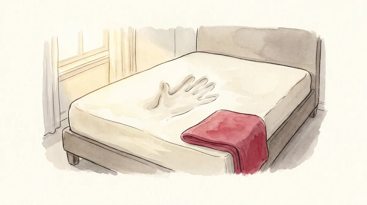
Press your hand into a memory-foam mattress. The foam gives instantly and a dent appears: that is the short run, where the push changes the shape of things. Hold still and watch: the foam creeps back, slowly, until the surface is flat again and only one thing has changed, the position of your hand against a recovered surface. That is the long run.
The economy is the mattress. A shock (a money expansion, a spending cut, an oil price jump) dents output first, because prices are sticky and cannot absorb it. Then prices gradually unstick, and as they adjust the dent heals: output creeps back to the size the pie chapters dictated, and the shock ends up absorbed entirely by the price level. AD-AS is the diagram of that healing, and it is the finale of the course:
In the cockpit you always flew at a fixed price level. Ask a new question: what would equilibrium income be at a different P? Tell it with people first. Suppose every price in the country were lower. Nobody printed a single new euro, but every euro already sitting in every wallet now stretches further: measured in stuff, the town is holding more purchasing power in cash than it meant to park at the old fee. You know this scene from Macro-05: everyone tries to un-park the extra, lenders get flooded with offers, the parking fee falls, more projects clear the bar, and the fountain fills. Lower prices ended up as higher spending, through nothing but the wallet math. In exam words, the chain reads:
P↓ → M/P↑ → LM right → r↓ → I↑ → Y↑
Lower prices, higher demand for output: plotted in (Y, P) space that is a downward-sloping curve, the aggregate demand curve AD. Every point on it is an IS-LM equilibrium; the curve is your whole cockpit, folded.
What shifts it? Exactly what shifted things in the cockpit. Fiscal policy (G↑ or T↓ pushes IS right → AD right). Monetary policy (M↑ pushes LM right → AD right). And any spending or money shock: the slides' example is a drop in velocity (people hold money tighter, spend less), which pulls AD left just like a money contraction.
Demand alone fixes nothing; you need to know what suppliers do. The course draws two supply curves for two time scales:
The bridge between them is one rule, straight from the slides:
| If in the short run... | then over time P will... |
|---|---|
| Y > Ȳ (economy running hot) | rise |
| Y < Ȳ (economy in a slump) | fall |
| Y = Ȳ | stay put |
And remember who actually does the adjusting, because it is nobody called "the economy". When Y sits above Ȳ, every firm in town is running hot: queues at the counters, waiting lists, overtime. As each catalog comes up for reprinting and each contract for renewal, each keeper does the shopkeeper thing you have now seen three times: raise the sign. When Y sits below Ȳ, it is unsold stock and empty tables instead, and the reprints go the other way. Price adjustment is that slow parade of reprints, and it is the force that walks the economy from its short-run equilibrium to its long-run one. You are about to drive that walk yourself.
The blue curve is AD, the amber line is the sticky short run (SRAS), the dark wall is the ch. 4 long run (LRAS at Ȳ = 1000). Hit the economy with a shock, read the dent, then press the green button and let time pass.
Expand M by 10% and fast-forward. Output visits 1100 and comes home to 1000; the price level ends exactly 10% higher; and behind the scenes M/P, and with it the interest rate, are back where they started. Money bought a temporary boom and a permanent price tag. That journey, frozen into four exam options, is mock-2 question 13.
Mock-2 question 13: horizontal SRAS, economy at its long-run equilibrium. M increases. What happens to r, Y, P in the short run, and then in the long run relative to that short run?
Short run (P frozen): more money → LM right → r falls, Y rises above Ȳ, P constant. The dent.
Long run (relative to the short-run moment): Y > Ȳ, so P rises; rising P shrinks M/P, LM slides back left, so r rises back and Y falls back to Ȳ. The spring-back.
Answer: SR: r decreases, Y increases, P constant; LR: P increases, Y decreases, r increases. Every AD-AS question is these two frames; the only work is keeping them in order.
Demand shocks dent the mattress from above. Supply shocks attack the foam itself: they change firms' costs and therefore the prices they charge. OPEC's oil embargo raised oil prices 11%, then 68%, then 16% across 1973-75; production costs jumped, firms passed them on, and the SRAS line itself lurched upward. Result, visible in the machine: prices up and output down at the same time. The 1970s data in the slides shows exactly that double hit, inflation and unemployment rising together (they even had a name for it, stagflation), and the mirror-image episode in the mid-1980s, when oil collapsed and both fell.
Now the dilemma. After an adverse oil shock the central banker holds two bad options:
Try both in the machine. This trade, pain now against prices forever, is what "stabilisation policy" means in practice, and it is the cliffhanger that Macro-07's Phillips curve turns into arithmetic.
From the exercise sheet: predict Y and P, both horizons, one shock at a time. Horizontal SRAS, economy starting at long-run equilibrium.
| Shock | Short run (P stuck) | Long run |
|---|---|---|
| M↑ or G↑ or T↓ (AD right) | Y↑, P same | Y back to Ȳ, P higher |
| M↓ or G↓ or T↑ (AD left) | Y↓, P same | Y back to Ȳ, P lower |
| Adverse supply shock (SRAS up) | Y↓, P↑ | back to original Y AND P (if CB waits) |
| ...accommodated by CB | Y restored fast | P permanently higher |
| AD slope logic | P↓ → M/P↑ → r↓ → I↑ → Y↑ |
| SRAS / LRAS | horizontal at P̄ / vertical at Ȳ = F(K̄, L̄) |
| The adjustment rule | Y > Ȳ: P rises · Y < Ȳ: P falls |
| Money in the long run | neutral: only P keeps the change |
Two frames per question: the dent, then the spring-back. That is the whole exam recipe.
Six questions, real mock-exam style: +1 right, −⅓ wrong, 0 skip.